We should measure effect sizes on substantively important scales

Why I'm still not a polygenic score nihilist

Both Sasha Gusev and Eric Turkheimer were kind enough to respond to my original post Why I Am Not A Polygenic Score Nihilist, Sasha in a comment on the post, and Professor Turkheimer in his own post.

It’s always nice for a writer to get attention from distinguished people. Eric Turkheimer is as distinguished as they come: he’s one of the two most important behaviour geneticists alive today, the other being Robert Plomin. (He also writes well and interestingly about the field on his Substack.)

But distinguished people aren’t always right, and it’s even nicer when their criticisms are dead wrong. Robert Plomin thinks “parents don’t make a difference” — yes they do —

— and here, Professor Turkheimer mischaracterizes my argument, ignores my substantive points, has a one-sided view of effect sizes, and makes one silly mistake. Most importantly, his argument will never, ever convince any neutral observer.

We are going to get into the weeds, but there’s an easy way to see why his argument will never be convincing. Just look again at this graph.

Turkheimer’s argument depends on persuading you that effects of this size are trivial and unimportant, because the R-squared of the variables (the polygenic score for educational attendance, and actual university attendance) is just 0.04.

But effects of that size are obviously huge and important! The difference between a 20% and a 50% chance of going to university is very, very big. Parents would give their eye teeth for a change that big for their offspring. Policymakers would spend billions to get it for their populations. And as a natural consequence of these facts, academics should get large grants to study it. Given that, if the R-squared is just 0.04, which it is, then… too bad for the R-squared!

(Both I and Professor Turkheimer agree that this graph isn’t the true causal effect and that the true causal effect is about half as much; I won’t keep mentioning this, but will just repeat what I’ve said extensively before, that the true causal effect is still very big.)

Turkheimer makes absolutely no points against this central argument. I’m not surprised, because I think it’s hard to deny. He does make one point against the graph above, which is that it doesn’t show the variation around the mean prediction:

The slope of the tops of the bars is that same unstandardized regression coefficient they keep estimating, but unlike a real scatter plot they have eliminated all the actual points around the regression line. They have eliminated the error in their prediction model by simply refusing to plot it.

We’ll consider that point in general below; but applied to the graph above, it is literally nonsense. The graph above shows a binary variable. It shows what proportion of each decile went to university: they either went, or they didn’t. The mean of a binary variable tells you everything about its distribution. In the bottom decile 17% of people went to university. For them, the “error” of the 0.17 mean is minus 0.83. For the other 83%, the error is plus 0.17. You needn’t plot anything else. There is nothing else to plot. The graph tells you all you need to know.¹

Actually, I used this as a joke in one of my presentations, so I may as well repeat it. Here’s a graph of the variation around the mean:

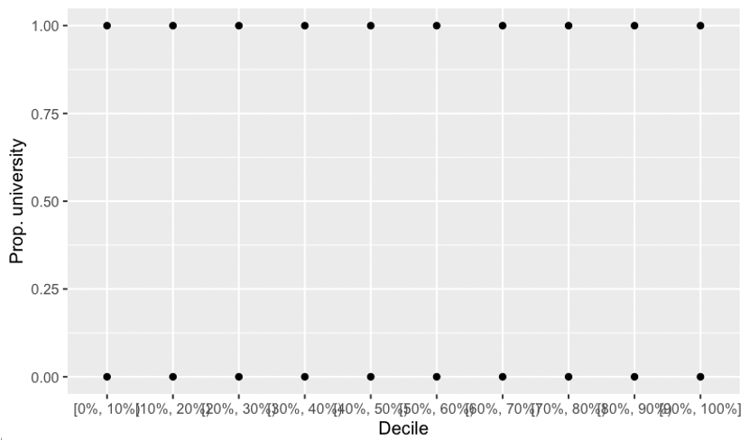
Happy now?²

Until you can convince parents and policymakers that a five, ten or fifteen percentage point change in going to university is not a big deal, you are never gonna win this one. Sorry.³

There are arguments that would be convincing! If you could show that the regressions within siblings somehow misestimate the causal effect of the polygenic score, or maybe overestimate the total causal effect of all genetic variation, then that would be persuasive. Or, maybe the UK Biobank sample used in the graph is very atypical, and for other samples, the same picture would show much less variation. That’s not impossible, though since UK Biobank respondents are more educated than the UK population of the same age, you’d expect variation to be dampened by range restriction, rather than exaggerated. More plausibly, effect sizes for other polygenic scores might be less substantively meaningful. If the causal effect for the polygenic score for ADHD moves the needle from 2% to 2.1% then sure, so much the worse for it. As I said before, what counts as substantively meaningful depends on what the dependent variable is. A change in suicide rates is different from the same change in self-reported unibrow. I’d be interested to see those arguments!

That is really all most people need to know. The rest of the article will get more nerdy.

Effect sizes, but which?

First, notice that Professor Turkheimer completely mischaracterizes my argument when he has me saying “effect sizes don’t matter”. That is just a weird take, when my entire article was focused on how the effect size of the PGS is really big. I just measured it on a different scale from what he wants! It’s as if I wanted to measure speed in miles per hour, he wanted to use kilometers per second, and he accused me of saying speed doesn’t matter.

What he seems to want is for everyone to use correlation coefficients as the only possible effect size: anything else shouldn’t count. And he writes down simulations to show that you can make the correlation arbitrarily small, while the effect size on a different scale stays the same. Funnily enough, I’ve written down almost identical simulations, to make just the same point. That suggests that these simulations aren’t going to settle the argument. After all, we already have real data where the R-squared is very low and yet the effect sizes on a different scale are large.

Now, sure, a correlation can be an effect size, if we know the direction of causality and have no worries about confounding. It then gives an effect size measured on a particular scale: the effect of a one standard deviation change in the independent variable, measured in standard deviations of the dependent variable.

Is that the only legitimate scale to use? Should we always measure things in standard deviations?

Well, first note that if so, my whole argument above about the graph must be wrong. Since it shows an R-squared of 0.04, and hence a correlation of 0.16, it must be a trivial effect size! Somebody should tell all those parents.

More broadly, consider this example. Suppose a drug is developed which gives everyone who takes it one extra year of life, exactly. Now, suppose that the drug is for sale in two communities, and in one community the standard deviation of life expectancy is twice as big as in the other. Should we say that in the first community, the drug’s effect size is half as much?

Of course not! What you get is always the same: one extra year of life, with its 365 extra days and four seasons.

There are certainly variables which it makes sense to measure in standard deviations. One is polygenic scores themselves! Polygenic scores, especially for binary outcomes like disease, are naturally scale-free. It makes complete sense to measure the effect of one standard deviation change, or equivalently, to standardize the score to have a mean of 0 and standard deviation of 1. And that’s just what I did in my article, talking about the effect of a one-standard deviation change in a PGS. It’s particularly sensible because PGS are very normally distributed, so researchers have a good intuitive sense of where one standard deviation takes you.

But there are many cases where it makes much less sense. First, it’s often quite unintuitive. This is especially true for binary variables like university attendance or disease. Here, a standard deviation is kind of a silly statistic: it can always be read off one-for-one from the mean, and it translates from an intuitive measurement (percentage probability) to a complex one. Quick, if 30% of people have a condition, how big is a one standard deviation change?

More seriously, standard deviations are often not the units that people care about, like in my drug example and in the education graph. If you are deciding what science should get done, then you should care about effect sizes on scales that matter to humans.

More seriously still, standard deviations, and therefore correlation coefficients and R-squared, can be very misleading when variables contain measurement error. Like, oh, every social science variable ever. One famous example: income. Income is a nightmare to measure. People think about their income on different scales, have irregular income which they don’t remember, misremember it even when it’s regular, share it with other household respondents in opaque ways, don’t know how much tax they pay, oh and they lie about it too. The UK Biobank, which takes the time to ask respondents whether they eat Scotch eggs, deals with this problem by ahahahahahaha asking a single five-category household income question (from “Less than £18,000 per year” to “More than £100,000”). Might there be measurement error? You think? A low R-squared explaining this variable, from genetics or anything else, doesn’t tell us a damn thing. A high R-squared would be informative, sure. It would tell you the researcher is cheating, or accidentally regressing something on itself.

In general, the problem with taking R-squared as a guide to importance is that some phenomena are inherently noisy. A model can have a low R-squared, and yet be entirely correct, identifying the only systematic factors that matter and correctly showing that everything else is noise. That’s why the best comparison is not an imaginary theory that explains 100% of the variation, but real alternative effects and how much they explain. And here, as I pointed out in my response to Sasha, there are few known environmental effects on university attendance that are as big as what genetics does, as captured in the “EA3” polygenic score.

Lastly, Professor Turkheimer makes a lot of appeals to history and authority: stuff about Pearson and “the entirety of ANOVA-based behavioral science”. Sorry, but there are entire disciplines which don’t use standardized effect sizes as a matter of course. In economics you rarely see them. Economists study behaviour too, they are not doing something fundamentally different from “ANOVA-based behavioral science”. And indeed, the use of R-squared is not some uncontroversial scientific pillar: it is profoundly disliked by many statisticians, for reasons related to my argument above. Here again is Cosma Shalizi. Some relevant excerpts:

“R2 can be arbitrarily low when the model is completely correct.” As in my point about measurement error.

“R2 can be arbitrarily close to 1 when the model is totally wrong.”

“R2 is also pretty useless as a measure of predictability.”

“R2 cannot be compared across data sets.” As in my example of the drug.

And on correlations:

“In 1954, the great statistician John W. Tukey wrote (Tukey, 1954, p. 721)

‘Does anyone know when the correlation coefficient is useful, as opposed to when it is used? If so, why not tell us?’

Sixty years later, the world is still waiting for a good answer.”

So, there’s no good case for correlations being a uniquely good measure of effect size, and the focus on them in behaviour genetics is a quirk of the discipline’s history, not something that all social scientists must bow to.

By the way, here’s a ChatGPT list of low-R-squared, yet important, results in social science. (I would have added democratic peace theory; wars are notoriously hard to predict, but the regularity that democracies fight fewer wars is deeply important if true.) Interestingly, it volunteers the interpretation: “Causal or policy relevance comes from the coefficient, not the fit.” Since obviously ChatGPT is smarter than all humans, this settles the debate :-)

When does variance matter, and variance of what?

Turkheimer is on stronger ground with the general point that variance around the mean matters. It is often fair and wise to ask how much variation there is around a conditional mean. But here too things are complicated.

Prediction: uncertain outcomes are not ignorable

First, are we doing prediction or causation? If we’re doing prediction, then indeed you want to know how accurate a polygenic score is. Again, this doesn’t imply R-squared is a good measure for that. My graph would have been a way to predict someone’s university attendance, at birth, from their DNA, and if you want to do that, there’s obvious value in distinguishing between a 20% and 50% chance of finishing university. (Not causal!) Ergo, if you think the R-squared of 0.04 proves the polygenic score is useless, you are just mistaken.

If you have enough data, you can get not just the conditional mean of an outcome based on a polygenic score, but the whole conditional distribution. Other things being equal, you’d always like more accurate predictions. But does that imply an inaccurate prediction is unimportant? Not necessarily. Think about income again. Suppose I have a low PGS predicting my income. In fact, the prediction is £20,000 per annum, with a standard deviation of £10,000. Meanwhile my sister has a high PGS and is predicted £200,000 per annum with the same standard deviation.

Now suppose a (mildly miraculous) new PGS is developed. We still have the same mean predicted income, but the standard deviation is now much smaller, let’s say zero! Do the differences in our scores now matter more? Or less?

On standard assumptions about the shape of the utility function with respect to money, I should be more worried by a mean income of £20K with a standard deviation of £10K, than by £20K for sure. (People are risk averse.) Also on fairly reasonable assumptions, my sister might be roughly equally relaxed about getting £200K for sure, or £200K plus or minus £20K-ish. (When you’re rich, maybe risk aversion becomes less important.) If so, then the information in the less accurate polygenic score might be more concerning.

This is a slightly wacky example, but I think there are plenty of outcomes where you’d get similar effects. Suppose your male child’s PGS predicts that his height will be 5 feet 6 inches. Would you be less worried if the lab assistant tells you “never mind, it might easily be 5 feet 10… or 5 feet 2”? In disease severity, we may be more interested in the chance of passing a certain threshold than in the mean.

My point is not that we shouldn’t try to be as accurate as possible. My point is that noisy predictions can still be informative and important.

Causation: noisy outcomes do not imply noisy effects

When we look at causation, things get more interesting.

The below plots thirty simulated data points under Control and Treatment conditions. The X marks the mean outcome in each condition, and the dots show the individual points varying around it.

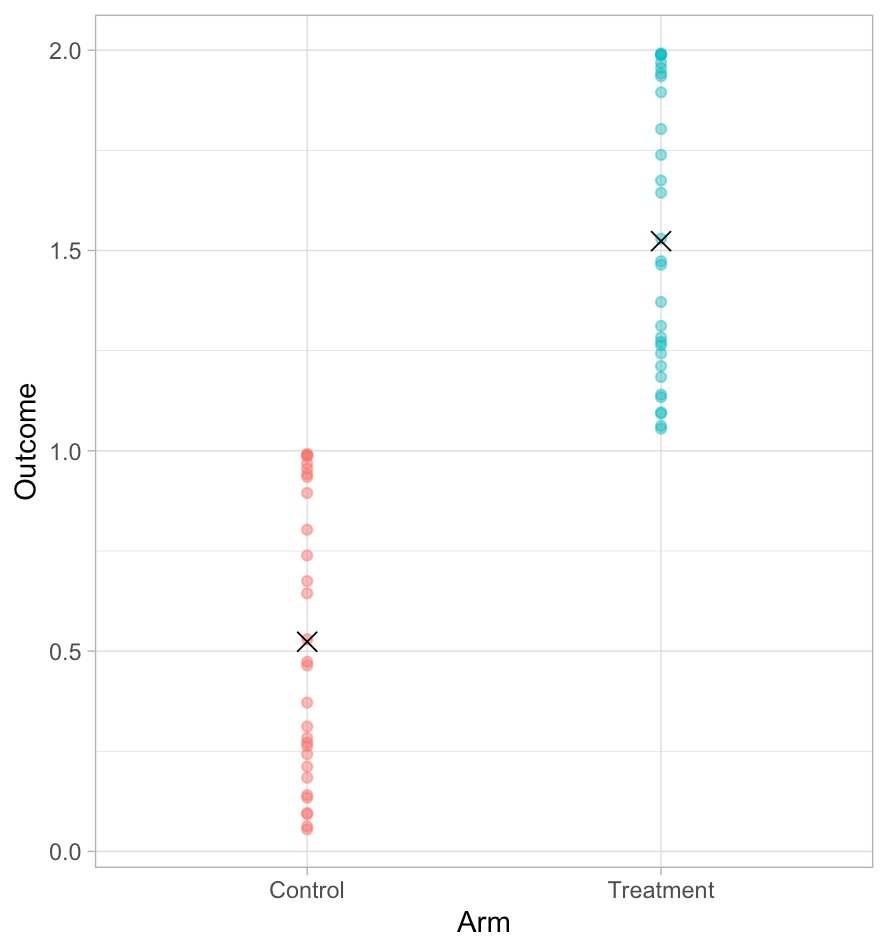
The average treatment effect — the difference between the Xs — is exactly 1. How much variation is there in that, though?

The picture doesn’t tell us. That’s because it could equally represent either of two cases. Here, I’ve joined up pairs of dots. Each pair represents one unit in each of the two conditions, the treatment and control.

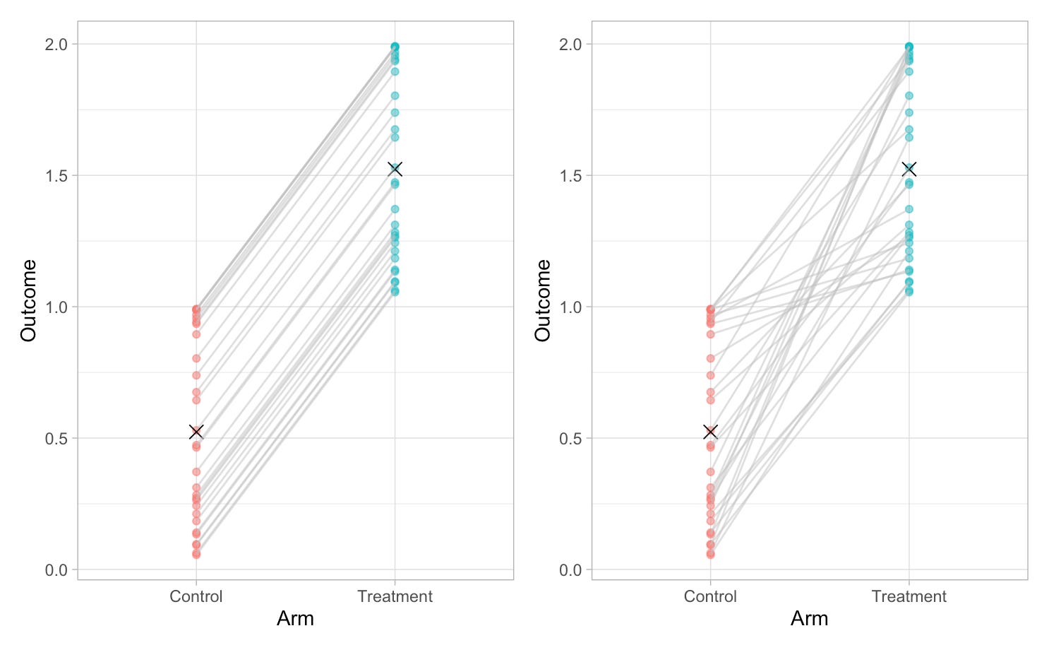
In the left hand picture, the effect of the treatment is always exactly 1, with no variation at all. In the right hand picture, there’s much more variation: the standard deviation of the treatment effect is about 0.5, and it ranges from 0.2 to 1.9.

In reality, we never have raw data like this: we only observe each case in one condition. We observe every person with the PGS they actually happened to get from their parents. If we do a scatterplot of outcomes against the PGS, the variation around the mean at any PGS value does not tell us about what would happen if any individual’s PGS were different.

Luckily, we have a paired natural experiment in sibling data. With full siblings, who have the same family, and genes allocated at random, you can draw a plot of differences in PGS against differences in outcomes — one dot for each sibling pair. This still isn’t good enough to tell you about the distribution of effect sizes, though. Each dot will give the difference in outcomes between a sibling pair, which will include both the effect of the PGS in that pair and random noise. The distribution of dots at any point on the x axis will be the distribution of the effect plus the noise. I don’t know a good way round this. Still, I’d like to see more such pictures.

But the key thing is that a picture of outcomes’ variation around the conditional mean, of the kind Turkheimer advocates for, still doesn’t tell you how effect sizes vary, which is the more interesting fact for many purposes. High variance in outcomes can be compatible with an extremely reliable effect size.

To apply this to education: sure, we see a lot of variation around the mean years of education, at every value of the PGS. But the effect of the PGS may still be quite reliable. We just don’t know.

Also, there is no reason to think that a change in PGS increases the variation. Suppose you were a parent considering embryo selection — not something I advocate, but it’s an easy way to clarify the issues. A child with a low PGS will get a low mean educational attainment (but with lots of variance). A child with a high PGS will get a high mean (with just as much variance). Why wouldn’t you choose the high PGS? You’re better off on average, and no more likely to have a very bad outcome. What this shows is that genetics can be consequential to decision-makers, even if there is a lot of noise.

Conclusion

The PGS skeptics have made hay with polygenic scores’ low R-squared, once the scores have been cleaned of noise from correlated environments. But at least in the case of education, a low R-squared is entirely compatible with effects that any policymaker or parent would think are large and important. To make their case, they need to show that in general, this is not true, rather than doubling down on how R-squared should override any other statistic.

This shouldn’t be hard to do! Just draw graphs of PGS against the outcome of interest, and then work out whether the change in outcomes is substantively important enough to warrant more research. You can certainly consider variation around the mean, too, or you can look at sibling pairs to make sure you’re capturing a causal effect. If all other PGS have substantively trivial effects, then I’ll be fine with that: I care most about educational attainment, because it’s so socially important. But show me how much real outcomes change.

1. In case you’re concerned about the deciles, they don’t matter either. You could plot percentiles or any other quantile and you’d get the same upward slope, maybe with a bit of a wiggle if the N in each quantile gets too low.

2. Could Turkheimer say that the underlying variable of educational attainment is the only important thing, and this could have different variances? Not really. University attendance is a known socially important variable in its own right, with all its benefits in terms of career access, future earnings, social networks and beer pong. And on the other hand, “educational attainment” measured in terms of years of schooling is a very rough measure of true educational attainment in terms of what a person has learned.

3. This isn’t just about parents’ subjective judgments. These effects would also be large in terms of objective statistics, like future earnings.